

Inference endpoint - When to scale up or down?
Inference endpoint scaling needs more capacity when requests wait in a queue and response time climbs. It needs less capacity when GPUs sit unused, and the cost per request rises without any traffic growth. This decision is different from scaling a normal web server. GPU memory and batch behaviour set the real limits here, not CPU usage. This guide walks through how a request moves inside an endpoint, which numbers tell you when to act, how to pick between replicas and a bigger GPU, the cost math to run first, and the five autoscaler settings that apply all of it automatically - the core settings behind any LLM inference autoscaling setup.
How does an inference endpoint process a request?
Understanding the internal path helps connect each scaling signal to its cause.
4 steps inside every request
Request enters the queue - A request arrives at the endpoint URL and waits in a queue. It stays there until the inference server has space to process it.
Server groups requests into a batch - The inference server pulls requests from the queue and groups them. How many groups at once is the batch size?
GPU processes the batch - GPU runs the batch and produces results. For language models, it streams tokens back to the user one by one as it generates them.
Results return to the caller - Endpoint sends the completed response back. For streaming responses, this starts before the full output is ready
3 terms that come up in every scaling decision
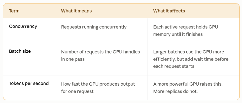
A queue that never clears is a concurrency problem. Slow individual responses are a tokens-per-second problem. Rising cost with flat traffic is a batch efficiency problem. Knowing which one you have decides which fix applies.
Why do GPU memory changes change the scaling rules?

A web server handles more traffic by adding CPU cores or instances. CPU utilisation at 70 to 80% is a reliable guide for when to act. GPU inference endpoints work differently for three reasons.
Model weights lock a fixed memory block
A 7B parameter model in FP16 precision uses exactly 14 GB of GPU memory. A 70B parameter model uses 140 GB. That block loads at startup and stays in memory for every request. On a 24 GB GPU like the A10G running a 7B model, roughly 10 GB remains for active requests. That remaining space sets the ceiling on how many requests one replica can handle at once, not compute power.
Each active request holds KV cache memory
As a language model generates tokens, it stores key-value pairs for every token it has processed in that request so far. A long conversation or a large context window fills this cache fast. On a memory-tight GPU, one request with a long context can block several shorter ones from starting because there is no cache space left for them.
High GPU utilisation is normal, not a warning sign
Production LLM endpoints typically run at 80 to 95% GPU utilisation during healthy operation. Token generation is compute-intensive by nature. A reading of 85% GPU utilisation does not mean the endpoint is overloaded. It is expected behaviour. The actual overload signals are queue depth, time to first token, and KV cache fill level.
This is why the metric table in the next section looks different from what most infrastructure teams use.
Which numbers tell you when to act?
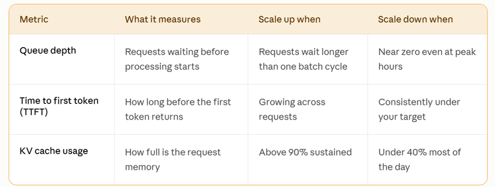
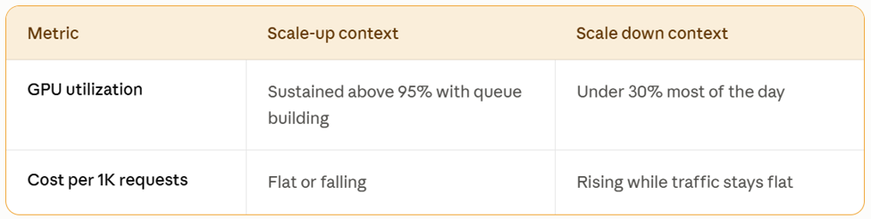
No single number gives the full picture. Check all 5 together - these are the core metrics behind effective GPU autoscaling.
Primary scaling signals
These 3 move first when the endpoint is under real pressure:
Secondary signals for context
These 2 do not trigger scaling on their own but confirm what the primary signals show:
Why queue depth and TTFT matter more than GPU utilisation?
GPU utilisation measures whether the GPU is busy, not how much more load it can take. A GPU at 87% utilization can already have requests queuing and TTFT tripling. By the time GPU utilisation reads as a problem, users have been waiting for a while. Queue depth and TTFT move earlier. It is the first number to check.
Why does p95 latency matter more than average latency?
It is the response time that 95% of requests fall under. Averages hide the slow tail completely. If 5% of requests take ten seconds while the average is one second, users experience the ten-second wait, not the average. p95 and p99 latency rise before averages do. Watch p95, not the mean.
Why is the cost per 1K requests rising, signalling a scale-down?
When traffic drops below the level where batches fill efficiently, the GPU runs at the same hourly cost but serves fewer requests per batch. Cost per request rises even though total traffic did not change. That is the clearest sign that capacity is more than the workload needs.
More replicas or a different GPU - How to decide?
The signals above point to a direction. This section decides the method.
Add more replicas
Add replicas when many requests arrive at the same time, and each individual request is fast. Queue depth grows, but TTFT stays reasonable on requests that do get through. One extra replica adds another full copy of the model in GPU memory and handles the concurrent requests that the first replica cannot reach.
Bigger GPU
Move to a bigger GPU when a single request is slow, the model barely fits in the current GPU's memory, or context windows are long. Adding more replicas gives more concurrency but does not speed up individual requests. A GPU with more memory and higher compute, for example, from an A10G to an H100, raises tokens per second and allows longer contexts without KV cache pressure. Before switching GPU types, compare tokens per second for your model across GPUs on InferenceBench - the throughput gap decides whether the H100's price premium pays for itself.
Smaller GPU
Move to a smaller GPU when a small model runs on hardware that is too large for it. A 7B model on an H100 at 15% utilization costs $3.50 per hour. The same model on an A10G serves the same traffic at $0.80 per hour.
Decision table
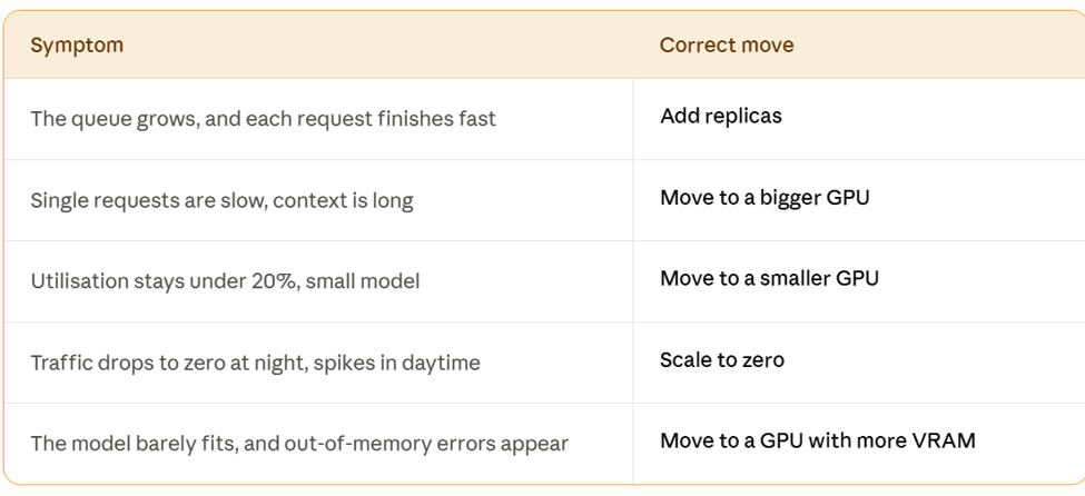
Before changing the GPU type, run the cost math below. Utilisation alone does not show which option costs less per request.
Cost math to run before changing anything
Formula
Cost per 1,000 requests = (GPU price per hour x number of replicas x hours running) divided by total requests served
Example A: Two A10G replicas
Two A10G replicas at $0.80/hr each, running 24 hours, serving 40,000 requests per day: (0.80 x 2 x 24) divided by 40,000 = $0.00096 per request
Example B: One H100
One H100 at $3.50/hr, running 24 hours, serving the same 40,000 requests: (3.50 x 1 x 24) divided by 40,000 = $0.0021 per request
What do the numbers show?
For this workload, two A10G replicas cost less per request than one H100. That changes when:
● The model needs the H100's larger memory to load at all
● Context windows fill the A10G's KV cache above 90%
● The H100's throughput advantage is large enough to close the price gap
Run this calculation before and after any GPU change. The number that matters is cost per request, not cost per hour.
5 Autoscaler settings that apply to all of this
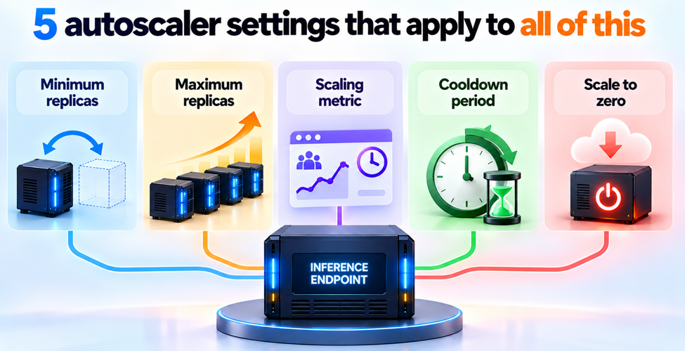
1. Minimum replicas
This is the floor. Setting it to zero means the endpoint shuts down when no requests arrive and costs nothing while idle. Setting it to one or more means requests never wait for a cold start, but idle cost continues through quiet periods. Deployment platforms like Yobibyte expose these five settings per endpoint, with publisher-verified recipes that set sane defaults for each model
2. Maximum replicas
This is the ceiling and the spending cap in one setting. Take the maximum acceptable hourly spend, divide by GPU price per hour, and set that number here.
3. Scaling metric
This decides what triggers a new replica to start.
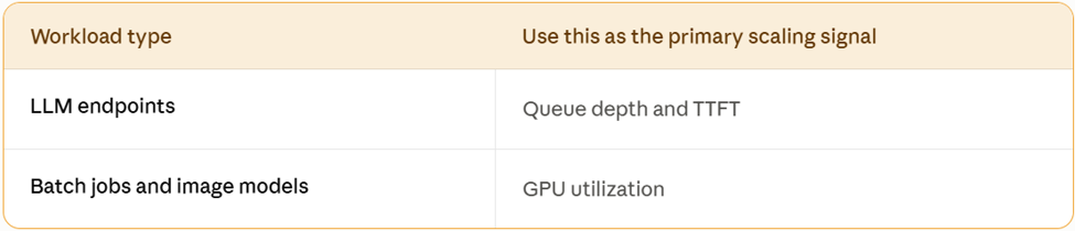
For LLM endpoints, queue depth and TTFT react faster. A surge in concurrent requests fills the KV cache before GPU utilisation moves. By the time utilisation climbs, the queue is already backing up.
4. Cooldown period
This is the gap the autoscaler waits between scaling actions. Without a cooldown, it adds and removes replicas in response to normal traffic variation. For LLM inference, five minutes is the recommended minimum for scale-down cooldown. Scale-up should react faster, within 60 seconds, so new replicas start before the queue grows large.
5. Scale to zero
This removes all replicas when traffic stops. The first request after idle waits for the model to load from storage.
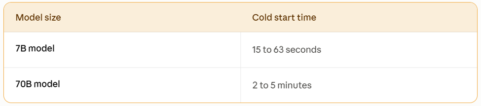
Pre-caching model weights on fast local storage cuts these times by up to 4x compared to loading from remote storage each time. If the first request cannot wait, keep a minimum of one replica.
Inference problems related to capacity are rarely loud. Before anyone calls it an outage, they demonstrate slow responses and climbing costs. It is not smarter teams that manage this well. They check fewer numbers more often and act on them sooner.
FAQ
How long does a cold start take?
A 7B model takes 15 to 63 seconds, depending on storage speed and whether weights are pre-cached. A 70B model takes 2 to 5 minutes. Pre-caching on fast local storage cuts load time by up to 4x.
Can scaling be scheduled instead of reactive?
Yes. Reactive autoscaling adds replicas after traffic arrives and latency climbs. Scheduled scaling adds replicas before a known peak. Both can run together: scheduled handles predictable peaks, reactive handles unexpected ones.
Do bigger batches replace scaling?
Batching raises throughput on the same GPU. At some point, traffic volume exceeds what any batch size can handle on one replica. Batching delays the need to scale but does not remove it.
Does scaling change the bill?
On per-request billing, cost follows traffic directly. On per-hour billing, cost follows replica count and GPU type. The cost formula above shows the full calculation for any setup.